Arxiv Dives
Arxiv Dives - Attention Is All You Need

Every Friday at Oxen.ai we host a paper club called "Arxiv Dives" to make us smarter Oxen 🐂 🧠. We believe diving into the details of research papers is the best way to build fundamental knowledge and keep up with the bleeding edge.
If you would like to join the discussion live, sign up here. Every week there are great minds from companies like Amazon, Doordash, Google, MIT, NVIDIA, Tesla, and many more.

The following are the notes from the live session. Feel free to follow along with the video for the full context.
Background
This is the start of a multipart series on Interpretability of Language Models. We received a lot of fascinating recommendations from the group in our discord.
A sub field of interpretability is “Mechanistic Interpretability”, or in other words - trying to interpret how each individual component of a transformer works and why.
Even the phrase "Mechanistic Interpretability" can feel intimidating. In order for any of it to make sense, we need to really pay close attention to…attention mechanisms 🤓.
Attention Is All You Need
Originally Published: June 12th, 2017 from Google, and University of Toronto
“Attention is All You Need” is the paper that everyone references as the seminal paper for Large Language Models.
Once we have this baseline understanding, we can work our way up to interpreting why the mechanisms work and how to improve them.
You’ve probably seen the diagrams and even read blog posts on Transformers.
In fact there are so many tutorials out there on how to write a transformer from scratch in PyTorch, GitHub copilot can complete the code for you as you define the modules. For fun, I decided to see how long it would take to simply click "enter" starting from a comment and create the full code for a transformer model.
Maybe we rename the paper to “Clicking Enter Is All You Need”.
Just kidding. There is a lot more to engineering a machine learning system than designing or implementing a model architecture.
Personally I like to think of models as "compilers" or "programs" and the data is what really drives them. A transformer could be applied to many different sequence prediction tasks, depending on what you feed it. So really it comes down to what data goes in and what data you want to come out.
Also...we can’t just let the AI do all the work for us! Otherwise we will never progress the research forward. Copilots today are really good at spitting out past ideas with not much innovative or new.
By the end of this, I hope you to empower you, to have an end to end understanding of what a transformer is, what attention is, and why it works so well. Diving into the basics is the best way to innovate.
Sequence Transduction
“Sequence transduction” is just a fancy phrase that means you are trying to predict an output sequence from an input sequence of different length.
For example, take translating Spanish to English.
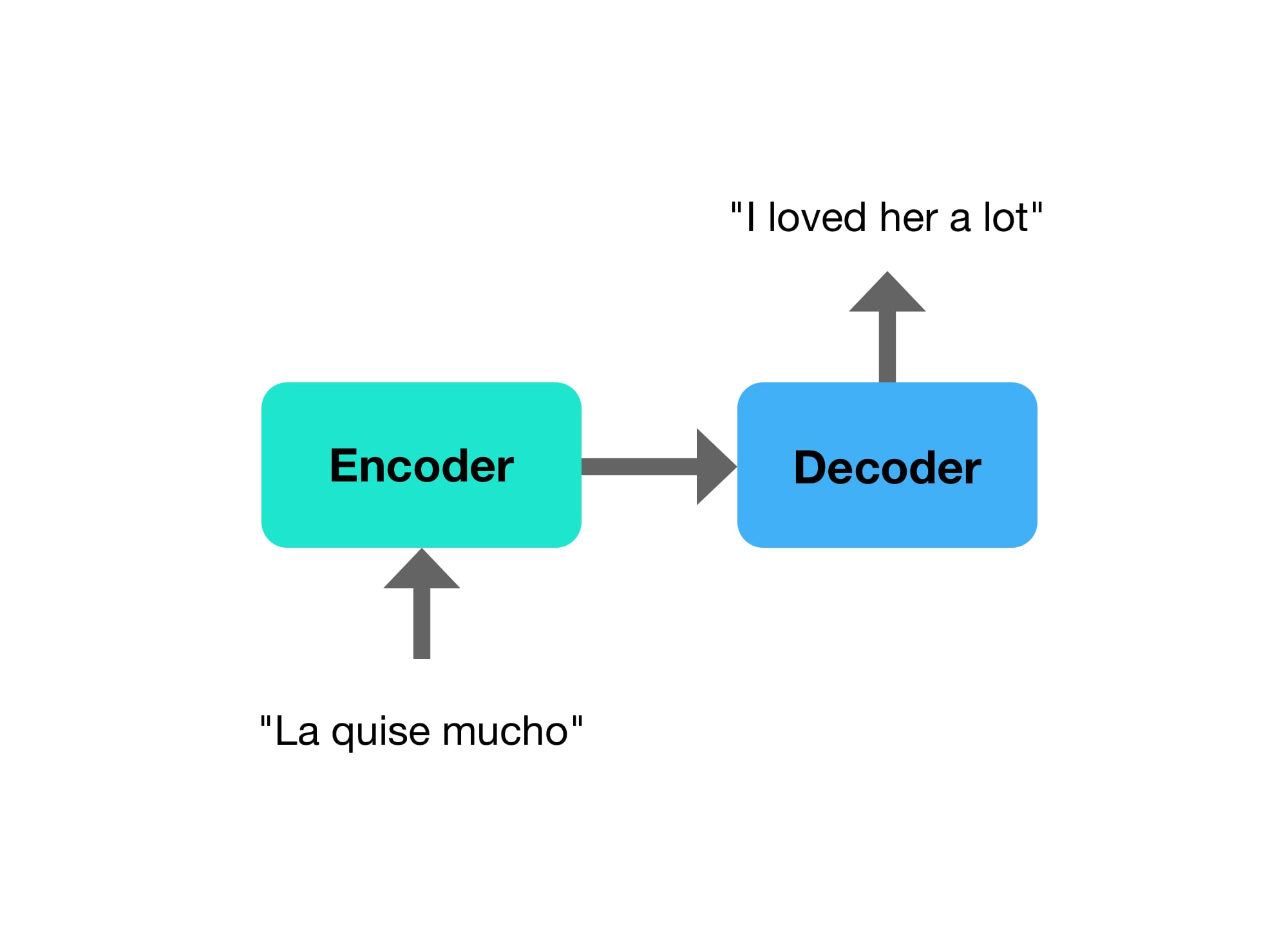
There is no guarantee that the input sequence is the same length, or even the same order as the output sentence. The first word in Spanish "La" corresponds to "her" in English, and there are 3 words in Spanish that translate to 5 words in English. There is clearly a need for fully reading the input before starting to translate the output.
You might also hear the decoding half of this called an “autoregressive” model.
In the before times (of 2013ish-2017ish) Convolutional Neural Networks (CNNs) and Recurrent Neural Networks were state of the art for “sequence transduction”.

As the title of the paper implies, they will be using an "Attention" mechanism to solve the sequence to sequence problem instead of the CNNs and RNNs.
Attention was not a new mechanism introduced in this paper. It was originally introduced as a component on top of other architectures to solve the problems with neural networks not being able to model dependencies in long sequences.
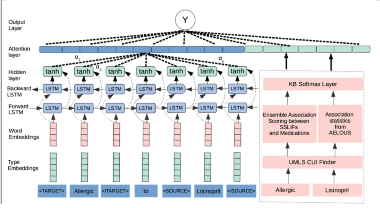
For example you might have had an LSTM + input features + Attention
It's also important to note that "Attention" can also be applied to computer vision, and is not limited to natural language.
Consider this crazy picture:

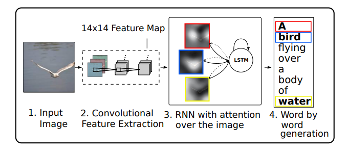
If you were to just consider the photo from the neck down, you may assume it was a person wearing a bandana, where in all actuality you need to attend to the whole image to see that it is in fact a dog. This may seem obvious to us, but computers are dumb, and need any clue they can get to solve problems like generating or describing an image like the above.
The “Show, Attend, Tell” paper from 2015 applied Attention in combination with an RNN to generate descriptions of images.
https://proceedings.mlr.press/v37/xuc15.pdf

Stacking all this complexity into a model gets quite expensive from a compute perspective, and also requires a lot of data for the end to end network to learn.
Key Takeaway
The key takeaway from this paper that they removed the recurrence and convolutions and introduce the Transformer based solely on Attention Mechanisms.
They apply the technique to Machine Translation of English-to-German and English-to-French, and show state of the art results after training for 3.5 days on 8 GPUs.
Note that now there are a few different types of transformers:
- Encoder Only - BERT
- Decoder Only - GPT
- Encoder-Decoder (or seq2seq) like the architecture we will discuss below.
Encoder-Decoder or Seq2seq is the most complex out of the three, because it combines and encoder and decoder, but if you understand Seq2Seq you will also understand the encoder and decode subsystems.
Model Architecture
Most competitive neural sequence models have an encoder-decoder model, where they encode an input sequence to a representation (or set of representations) and then decode those representations to an output sequence.
The diagram in the paper of the architecture made my eyes glaze over the first time I saw it, and to be honest, still does.
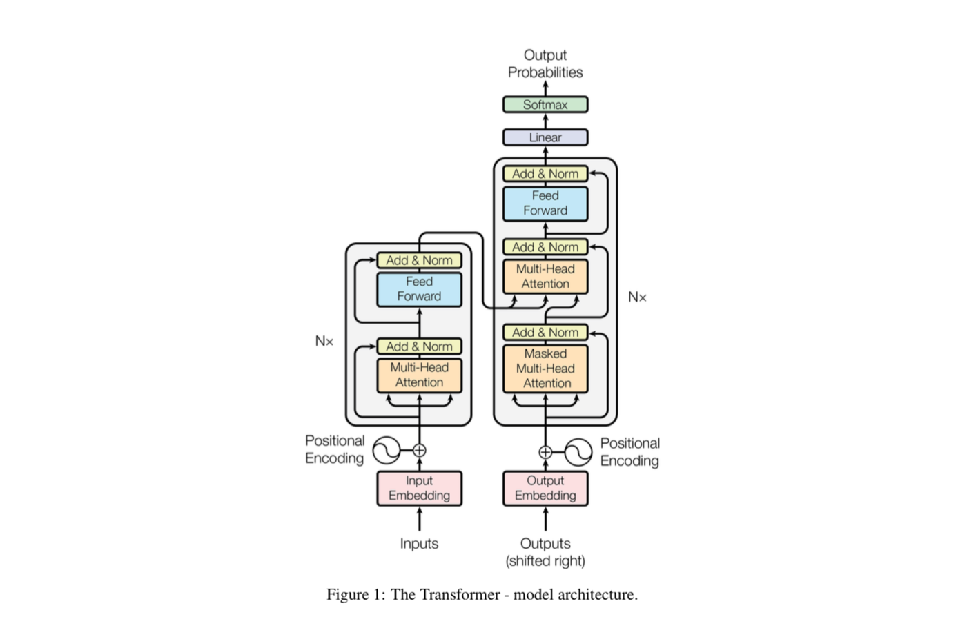
To fully understand it, we will break down each sub section piece by piece, zoom back out to the full diagram over and over again.
Input (Word) Embeddings
We will start at the bottom with the input and output embeddings.

First the encoder and the decoder takes in a set of input embeddings that represent each token. You can think of “token” and “word” as interchangeable here for simplicity sake.
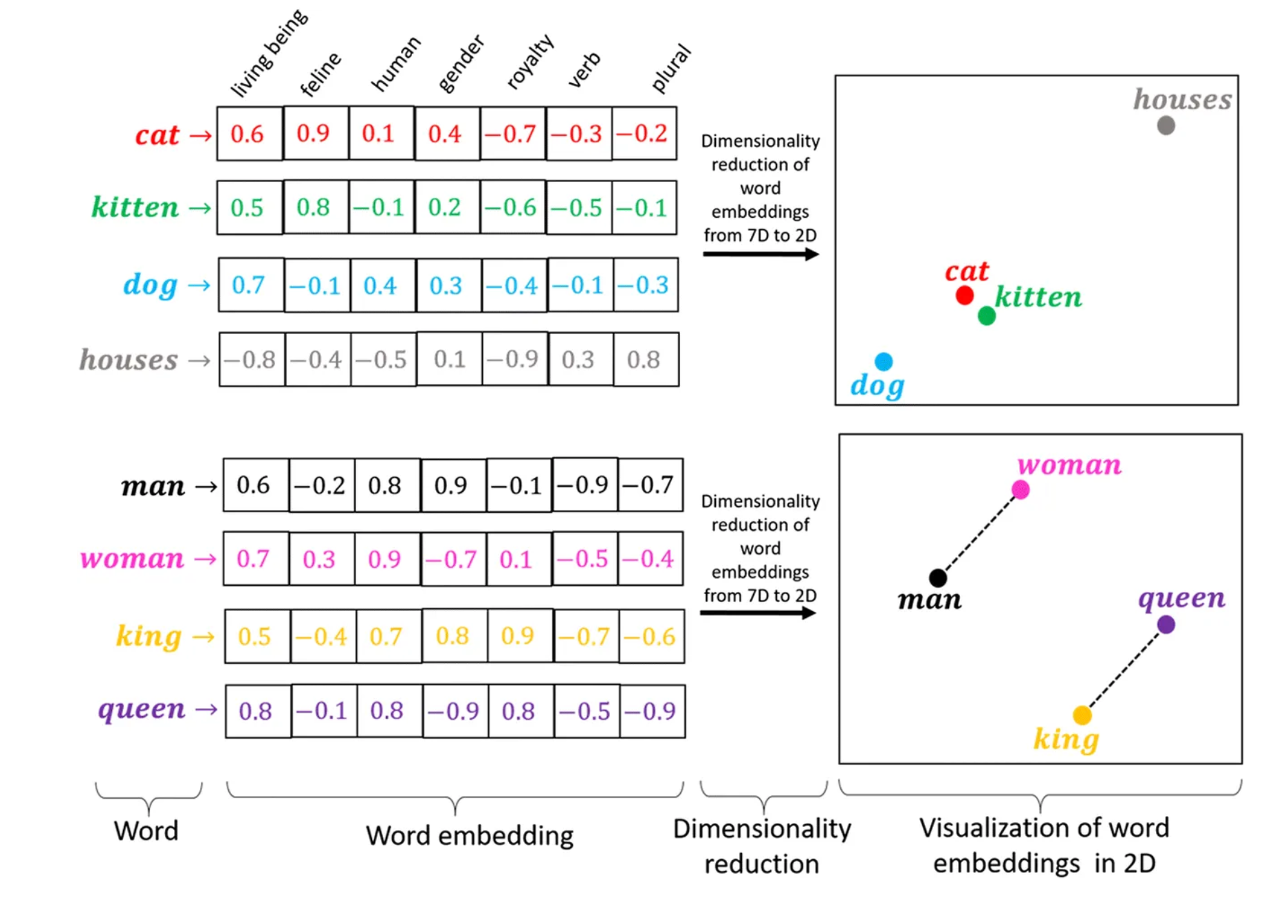
Words have complex meaning that can be represented as a distributed vector of numbers. We could have a whole dive on how they are created during training or pre-training, but here is a high level view of what they are trying to capture.
The Encoder
The word embeddings are then fed up to the encoder module.
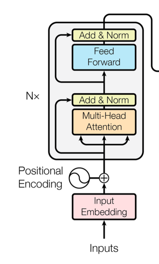
Ignore the position encoding and the inner details of the encoder for now, we will return to them later.
The encoder’s job is to look at the whole sentence, and decide what each word means.

In the case the encoder needs to process the three word embeddings for "La", "quise" and "mucho" so that they can be presented to the decoder.
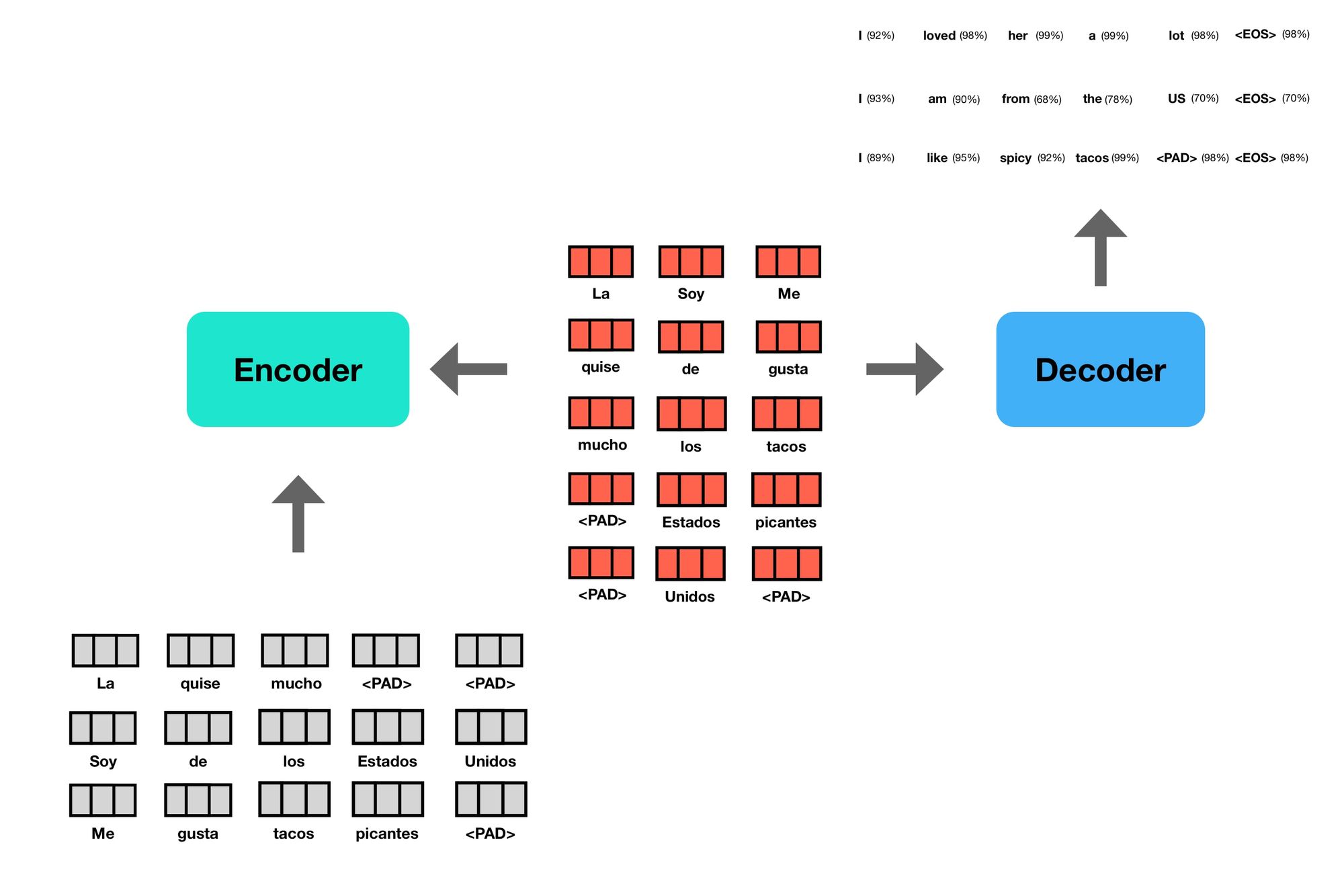
In practice, sentences are batched together by length, and the model can translate many sentences at once. This requires you add a token to ensure they are all the same length. This takes advantage of parallelization on the GPU during training and inference.
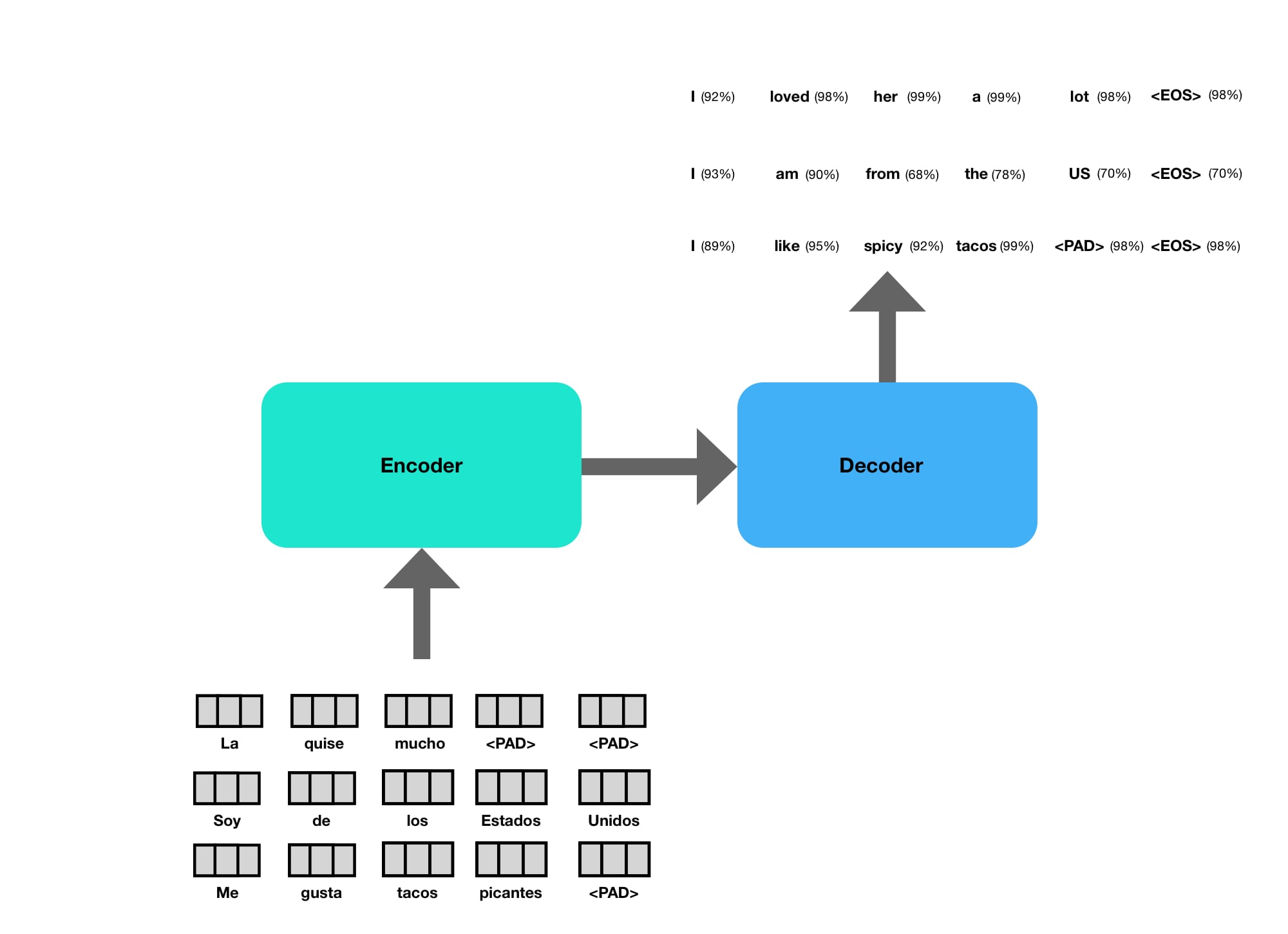
It is also common to have an “End of Sentence” (EOS) token in the outputs to tell it when to stop.
You can think of the connection between the two as a new set of word embeddings, with slightly different meanings. We’ll dive into why this is the case in a sec.
The Decoder
The decoder then takes in a processed representations, as well as previously generated word embeddings, and outputs probabilities for each word in the output.
The decoder outputs one token at a time. During decoding, the previously generated token becomes the subsequent input to the decoder.
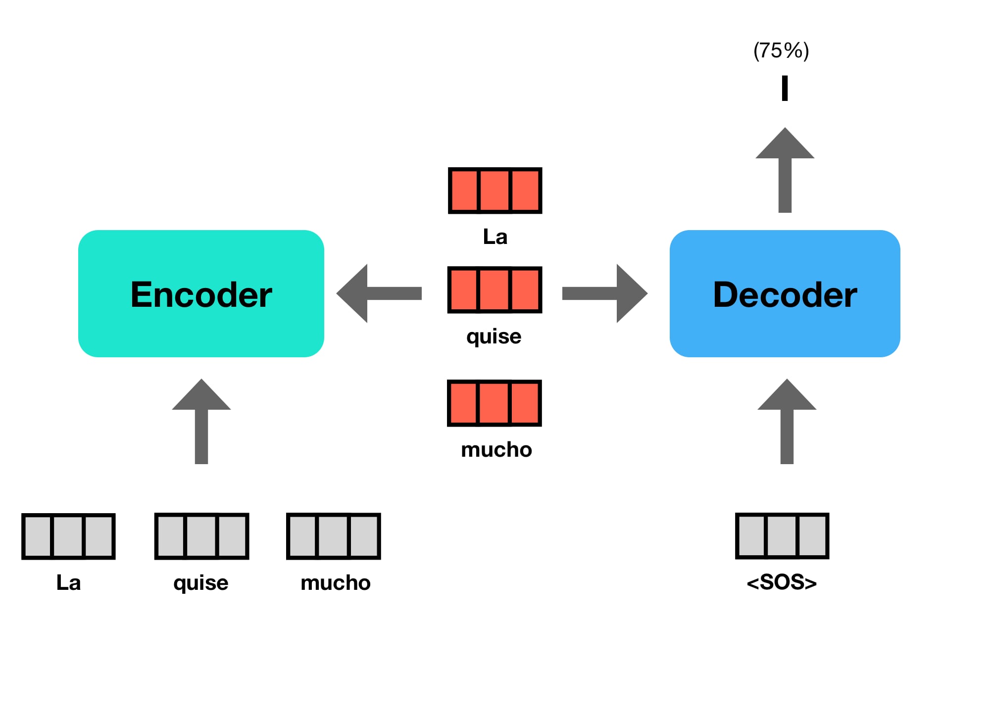
Since there is no previous token to start, the process is kicked off with a “Start Of Sentence” (SOS) token.
This type of sequential processing, using the previous outputs as new inputs is called an “autoregressive” model.
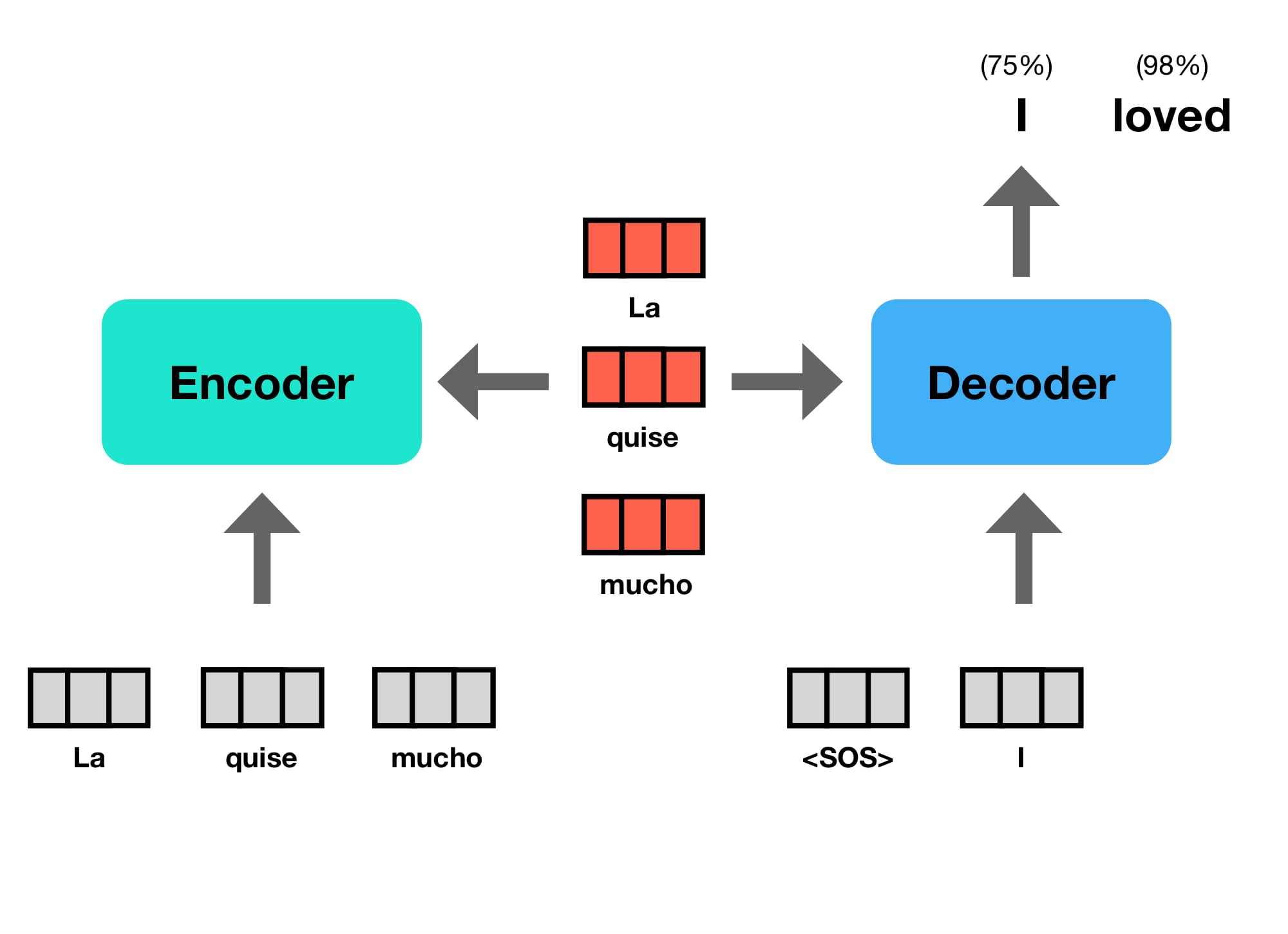
As you can see, after the model generates ("I") from ("<SOS>"), it then feeds ("<SOS>", "I") back into the model to generate ("I", "loved"), and so on and so forth.
A fun and practical fact is that the input and output embeddings can be shared, since they are using what is called a byte-pair encoding. Tokens are really substrings of full words, and if both languages are latin, you can use the same set of substrings.
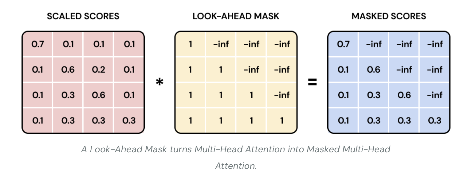
The decoder has to mask the future outputs so that it cannot “peek ahead” during training at all of the outputs because that would be cheating. So when you see “masked multi head attention”, that’s all this means.
This won’t fully make sense until we look at attention, but keep in the back of your mind.
The diagram in the paper makes it seem like there is just one encoder layer and two decoder layers. But in actuality they stack 6 encoders and 6 decoders on top of each other within that simplified diagram.

Back to the full diagram
Then within each one of the layers of the encoder and the decoder there is a set of "Multi-Head Attention Mechanisms" and "Feed Forward" layers.
You can see that the decoder has two sets of attention mechanisms, one that looks at itself, and one that looks at the outputs from the encoder.
The encoder simply as one attention mechanism that attends to "itself".
Attention
We've been throwing around this word "attention" but what is it and why is it “all we need”?
In natural language processing, words can mean different things in different contexts. A word embedding holds a lot of information about a word, but depending on the context, will shift in meaning.
Take for example the word “fly”. It can mean “fly an airplane” or “that fly is an annoying bug”. In one instance it is a noun, in the other it is a verb. Completely different meanings depending on the sentence.
If we just plot the word embedding itself, you can see for this set of embeddings, it is is much closer to the verb representation than the noun.
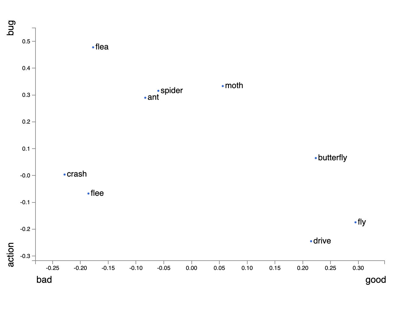
I was trying to think of what corpus might cause it to be closer to a bug representation, but the fact that “flies” “fly” around, means it will probably always be closer to a verb than a noun, unless you look at the surrounding words in a sentence.
Attention is used to solve this problem of disambiguation of words. It “looks” at different parts of the sentence, and shift the representation of words accordingly.
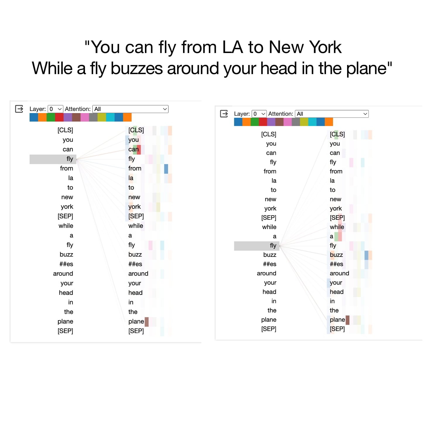
There is a fun demo on Google Collab where you can play around with the attention mechanism called BertViz.
You can see in the following sentence, the first instance of "fly" is a verb, and attends closely to the word "can" before it, "from" after it, and the locations you are flying to. While the second instance of "fly" is more interested in the words "buzz" and "while a". If you think of it, you can pretty quickly disambiguate a noun from a verb with "a fly" versus "can fly".
Queries, Keys, Values
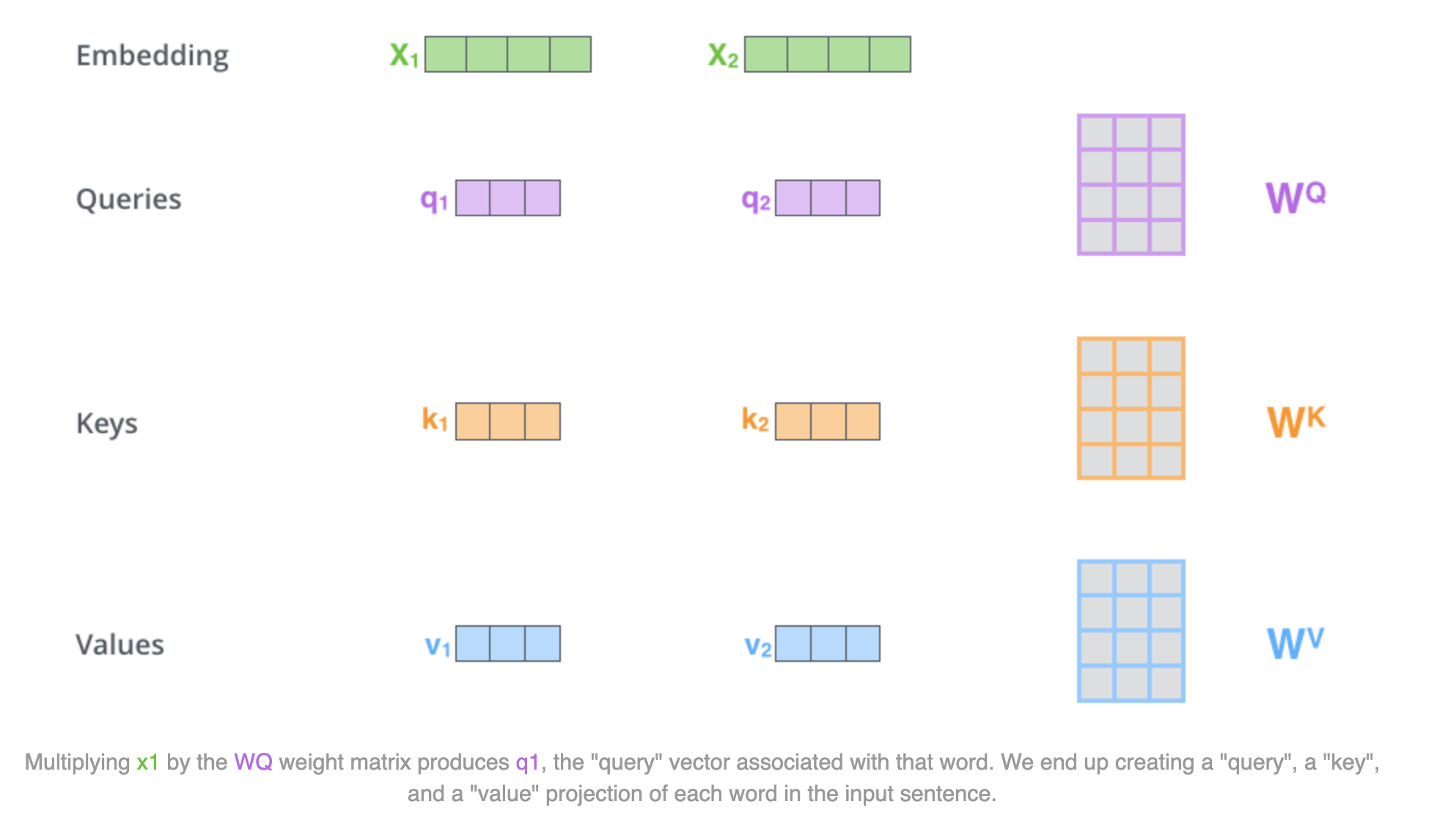
Attention in this paper is described as mapping a “query” and a set of “key” “value” pairs to an output.
Each word in the sentence has a corresponding a “query”, “key”, “value”, and “output” vector, that is computed given a set of weights.
The names query, key and value are inspired by information retrieval systems, where you might have one “query” as input, and you have to use it while you scan a bunch of items (keys) and select an item (value).
An analogy is you are in a grocery store isle, and you have a recipe with ingredients. Each ingredient is a query, each item on the shelf is a key, and each item you select is a value.
You can visualize this as when looking at the word “fly” (query) scan all the words in the sentence (keys) and select the most important words (values) that distinguish this particular meaning.
Since all of the queries and keys can be thought of as word vectors plus information about their position (see positional encoding later), you can think of “fly” sending it’s query out to all the other words saying “I am the word ‘fly’ in position 3, I am looking for surrounding prepositions or auxiliary verbs that may influence whether I am a noun or a verb”.
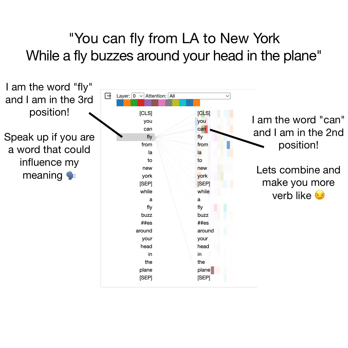
Then for each of the keys, they say “Hey, I am the word ‘can’ and I am right before you! Let’s get together and make you more verb like”. When you do the dot product between them, the combine their knowledge into one vector that is a more verb like version of “fly”.
Scaled Dot Product
The way Attention combines the words is through the “scaled dot product” of all the queries, keys, and values.
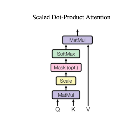
First multiply the Query and the Key together, scale them, run them through a softmax to see which other words are more important.
Then multiply the output of the softmax of Q and K by V to get the output meanings of each word.
The “output” is a weighted sum of the “values”, or the new representation of that word, in the context of the sentence.

Each step is relatively straight forward once you zoom in, but does get complicated as you zoom out. This is why Mechanistic Interpretability is interesting to zoom into the individual pieces and what they are doing.
Multi-Head Attention
If you simply did one layer of attention, you might reduce the amount of information and “decision making” that could flow through the network.
What this means in practice is that one layer of attention might get really good at grammar and parts of speech but one might be lack the ability to on disambiguate names from places (which are both nouns).
To solve for this, they add multiple attention modules, and let each one learn different patterns. Each one of these modules is called an “attention head”.
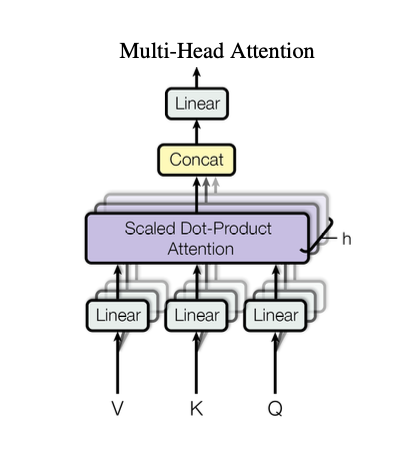
They call this attending to “information from different representation sub spaces” and claim that a single attention head would have a hard time attending to all the information present.
They then concatenate all the attention heads, and project the final values once again through a linear layer.
In the original model they used 8 attention heads, with dimension of 64 each.
Applications of Attention
There are a few places within the model that Attention is used.
- Communication between the encoder and decoder layers, where the “queries” come from the decoder, and look at the “keys” and “values” from the output of the encoder.
- The encoder attends to itself, all positions in the encoder attend to all positions in the previous layer of the encoder.
- The decoder attends to itself, but it has to mask information from being passed forward during training so that it cannot peek at the future. Because during inference it will only see each token at a time.
Feed Forward Networks On Top Of Attention
In addition to the attention layers, each layer contains a fully connected feed forward layer.
They are two linear layers with ReLU activations in between, as well as layer normalization. You can play around with other standard neural network architecture tricks in here, they kept it pretty simple.

Positional Encoding
Zooming back in to the bottom, you may remember there is a positional encoding that is added to each embedding.
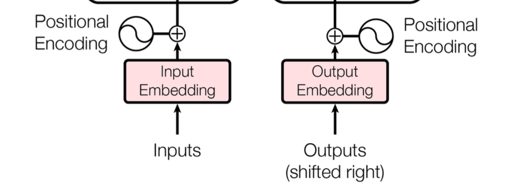
There is no inherent order when feeding in the embeddings to the model. This is a nice property because then you can calculate all the keys, queries, values, etc in parallel.
Since there is no order, there the model must enrich each input embedding with information about where it is. They inject information about the absolute position of each token in the sequence with a "positional encoding"
They do this with sine or cosine functions with different frequencies.

Concretely they take a positional encoding for each time step and add it to the word vector at each time step.
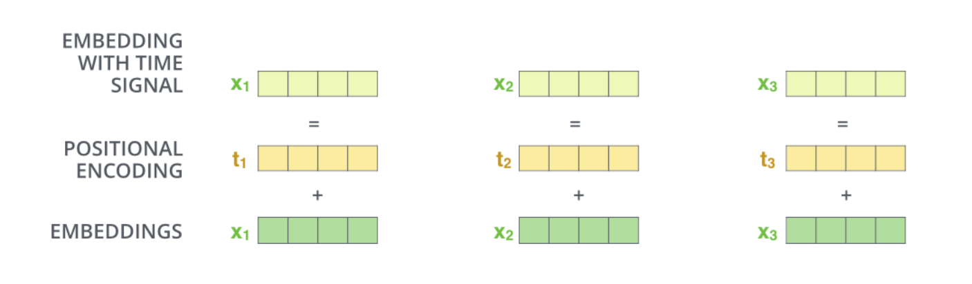
To visualize this, each row here is a positional vector that gets added to the word vector itself.

Why is Self-Attention Efficient?
You may be looking at the attention mechanism and thinking, well that is still a lot of computations at each step, why is this so much more efficient than a CNN or RNN?
Computationally, is N^2 in the size of your input and output sequences.
They compare self attention to the recurrent and convolutional layers for mapping one sequence to another sequence of equal length in Table 1 of the paper.
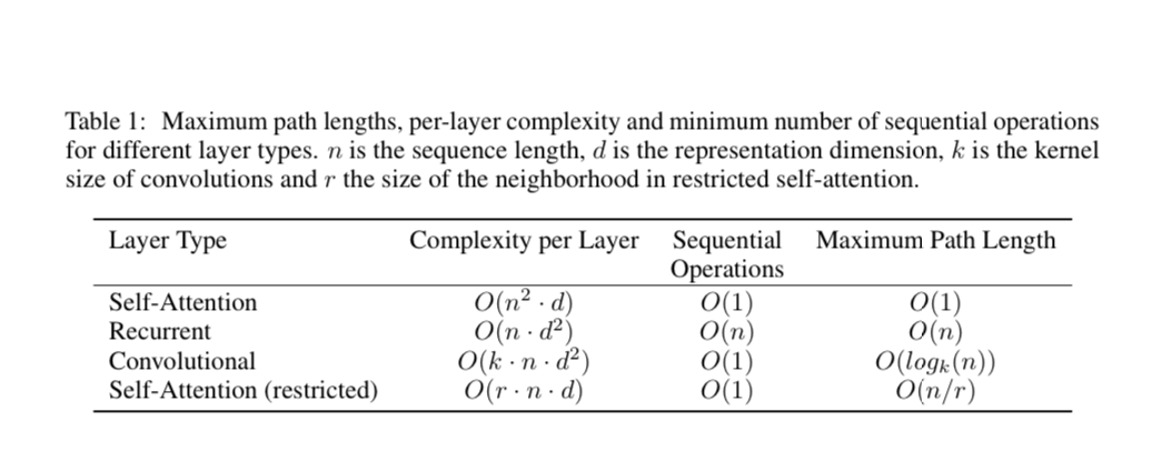
Three things they take into account:
- The total computation per layer
- The amount of computation that can be parallelized
- The path length between long range dependencies
The self-attention layer connects all positions with each other directly, meaning the path length is O(1)
It does not do not rely on the sequence being processed sequentially like a recurrent network which has O(n) sequential operations.
Since it has to connect each position with itself you get O(n^2 * d) in the complexity per layer, which is more efficient than squaring the dimensionality of each layer, because usually dimensionality is larger than the sequence length.
They consider the ideal of “restricted self-attention” where self-attention is restricted to a neighborhood of size r in the sequence centered around the respective output position and divide n/r to make it more linear, but save this for future work. (Has anyone seen this tried?)
Convolutional layers have to pass information from local regions by stacking layers with a kernel width of k, and doing so requires stacking O(n/k) so they are more expensive than recurrent layers. Some people fix this with dilated convolutions (skipping elements within a kernel).
They also propose it could help with interpretability, which we will dive into in upcoming dives.
Training
They used the WMT (Workshop on Machine Translation) English-German dataset with 4.5 million sentence pairs.
Below is an example of what the data might look like for an English to Spanish translation task.
https://www.oxen.ai/ox/WMT/file/english-spanish/data/es-en/commoncrawl.tsv?page=1&page_size=100
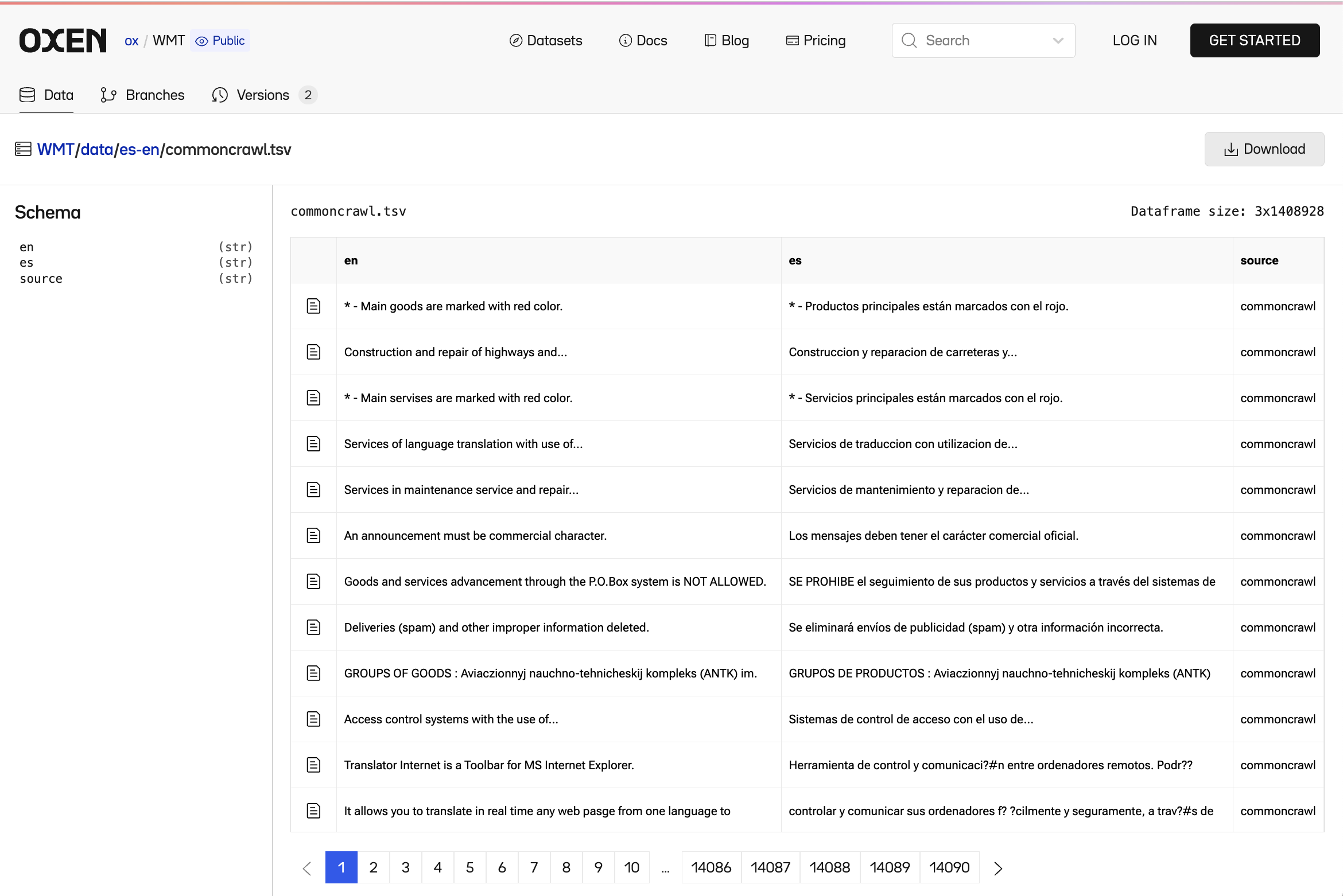
They used byte-pair encoding which has the same shared vocabulary of 37000 tokens, which means they can share the embeddings for the encoder and the decoder.
For English - French they used a larger dataset of 36 million sentences, with a vocabulary of 32000 word pieces (distinct tokens).
Sentences were batched together by approximate sequence length, each batch contained approximately 25000 source tokens to 25000 target tokens, which is a pretty large batch, need to do the math on how many examples per batch this might be on average.
They used 8 NVIDIA P100 GPUs, and trained the base model for 12 hours. Each batch took about 1.0 seconds to compute, and the large models were trained for 300,000 steps or 3.5 days.
Results
They evaluated on the “news” test set from the 2014 WMT challenge.
They also experiment with many different model configurations and sizes.

English Constituency Parsing
They explore the generalizability of the Transformer to constituency parsing, which is a task with highly structured outputs.
What is constituency parsing?
Starting with words that need to be classified into parts of speech. Then grouping words into phrases, where the phrases have categories (Noun Phrase, Verb Phrase). Then recursively group phrases into bigger phrases.

They train a 4-layer transformer with size of 1024 on the Wall Street Journal (WSJ) portion of Penn Treebank, which is an annotated dataset of constituency parses. There are about 40k sentences.
They also trained it off our the output of high confidence parses from the BerkleyParser corpora with 17 million sentences.
WSJ Vocab: 16k tokens
BerkleyParser Vocab: 32k tokens
Remember, the number of tokens influences the size of the embedding lookup layer, and hence the size of the model.
They held out section 23 of the WSJ dataset to evaluate on.
The results show that the model performs surprisingly well on this task, without the model being explicitly designed for this task.
Here is an example of the complexity, and structure of the output:

Conclusion
They introduce the transformer, a sequence to sequence model based entirely on attention.
The transformer can be trained significantly faster than previous RNNs or CNNs for sequence to sequence tasks and achieved a new state of the art on machine translation.
They mention that these models could extend well to input and output in other modalities such as images, audio and video, which we are seeing more and more of today.
Join the Herd 🐂 🌾
If you enjoyed this deep dive and want to join us live, sign up here: http://lu.ma/oxenbookclub?ref=blog.oxen.ai or join our discord: https://discord.com/invite/s3tBEn7Ptg
We would love to have you as a part of the discussion and help pick future topics to dive into.
Who is Oxen.ai?
Oxen.ai is an open source project aimed at solving some of the challenges with iterating on and curating machine learning datasets. At its core Oxen is a lightning fast data version control tool optimized for large unstructured datasets. We are currently working on collaboration workflows to enable the high quality, curated public and private data repositories to advance the field of AI, while keeping all the data accessible and auditable.
If you would like to learn more, star us on GitHub or head to Oxen.ai and create an account.